A Holistic View of the Determinant
Will Healy September 2026
Motivation
I wanted to write this essay because I think building an understanding of the determinant is so easy to skip when learning linear algebra. It is easy to skip because most elementary usecases of these concepts don’t really require a deep understanding of its meaning. I skipped taking time to understand the determinant when I first learned linear algebra. I didn’t think it was that important. When I started studying higher level math and ML, though, my lack of understanding was shoved in my face. For example I was very humbled when I was expected to quickly understand why $log(Det(X))$ was a convex function in a class full of PhDs. I realized I could barely define what the determinant really was. I then invested considerable time into understanding the determinant. I hope to share the intuitions I’ve built along the way. I also hope to present these in a way which is very clear and accessible, and bridges both the algebraic and geometric interpretations.
Multi-Dimensional Measures of Size
The determinant and trace can both be thought of as a multi-dimensional extension of magnitude. For a $1x1$ matrix $A_1$, also known as a scalar, the trace is equal to the determinant which is equal the scalar’s value. For a $2x2$ matrix, call it $A_2$, the determinant and trace are no longer equal (though they can be). They both still measure the size of the matrix, but they do so in different ways: determinant measures size multiplicatively whereas trace measures size additively. We will explain what this means for the determinant in more detail, but to quickly have some understanding of this statement note that for a matrix $A \in R^{nxn}$:
\[Det(2A) = 2^nDet(A) \\\] \[Tr(2A) = 2Tr(a)\]This essay will be structured in the following way. I will first define the determinant. This will take some time as the definition requires some prerequisites. I will then show several properties of the determinant which follow from this definition, optimizing for connecting the determinant to a breadth of other linear algebra concepts you may already be familiar with. Finally, I will show the determinant’s meaning geometrically, ending with an incredible result about the volume of sets. The goal is to build a holistic view of this function in a way which is impossible to forget.
Determinant
The determinant of a matrix is a metric which represents multiplicative magnitude. We will define it for a square matrix as the following:
The unique alternating m-linear function over $R^n$ which has the property of $Det(e_1, e_2, … e_m) = 1$
Let’s first understand this definition.
M-linear functions
An m-linear function is a function f of m variables with the following properties:
\[\begin{aligned} f(cx_1, x_2, ... x_m) &= cf(x_1, x_2, ... x_m) \\ f(x_1, cx_2, ... x_m) &= cf(x_1, x_2, ... x_m) \\ f(y_1 + y_2, x_2, ... x_m) &= f(y_1, x_2, ... x_m) + f(y_2, x_2, ... x_m) \\ \end{aligned}\]That is, it is linear with respect to each element in the input. So, multiplying an input by a constant while leaving the rest of the inputs alone multiplies the output by a constant. Additionally, the linear property of
\[f(a + b) = f(a) + f(b)\]holds for each input individually.
Alternating m-linear function
An alternating m-linear function is an m-linear function with the property that if two inputs are equal the output is $0$. The presence of this property implies another property, which is that swapping two inputs flips the sign of the output. To see why, let’s imagine we have a duplicate input $v$:
\[f(x_1, x_2, ... v, ... v, ... x_m) = 0\]This is $0$ by the definition of an alternating function. Now let’s decompose $v$ into two vectors:
\[v = u + w\]And thus,
\[f(x_1, x_2, ... u + w, ... u + w, ... x_m) = 0\]By the properties of m-linear functions we can decompose this into:
\[\begin{aligned} f(x_1, x_2, ... u + w, ... u + w, ... x_m) &= \\ f(x_1, x_2, ... u, ... u, ... x_m) &+ \\ f(x_1, x_2, ... w, ... w, ... x_m) &+ \\ f(x_1, x_2, ... w, ... u, ... x_m) &+ \\ f(x_1, x_2, ... u, ... w, ... x_m) \end{aligned}\]Since our assumption is that duplicate inputs equal $0$, the first two terms must be $0$ since both repeat an input. Thus, it must be the case that:
\[\begin{aligned} f(x_1, x_2, ... w, ... u, ... x_m) + f(x_1, x_2, ... u, ... w, ... x_m) = 0 \end{aligned}\]and so
\[\begin{aligned} f(x_1, x_2, ... w, ... u, ... x_m) = -f(x_1, x_2, ... u, ... w, ... x_m) \end{aligned}\]So, a function where duplicate inputs gurantee an output of $0$ implies that swapping two inputs negates the output. This will be an important property of the determinant.
One other result of an alternating m-linear function is that if the inputs are not linearly independent, meaning some input can be written as a linear combination of other inputs, then the output is $0$. To see why this is the case, imagine you have an m-linear function $f(x_ 1, x_2, … x_m)$ and you have an $x_i$ which can be written as a linear combination of the other inputs:
\[x_i = \sum_{j\neq i}^m a_jx_j\]Then, our function could be expressed as:
\[\begin{aligned} f(x_1, x_2, .., \sum_{j\neq i}^m a_jx_j,.. x_m) = \\ f(x_1, x_2, .., a_1x_1,.. x_m) + f(x_ 1, x_2, .., a_2x_2,.. x_m) + .. + f(x_1, x_2, .., a_mx_m,.. x_m) = \\ a_1f(x_1, x_2, ..,x_1,.. x_m) + a_2f(x_ 1, x_2, .., x_2,.. x_m) + .. + a_mf(x_1, x_2, .., x_m,.. x_m) = \\ 0 \end{aligned}\]This is $0$ since duplicate inputs yield $0$ output by the definition of alternating functions.
To summarize, we have shown three properties of alternating m-linear functions, one of which we stated as its definition:
- If two elements are equal, the output is $0$.
- If you swap two inputs, the output is negated.
- If the inputs are not linearly independent, the output is $0$.
Basis Vectors as Inputs Yielding 1
The last condition in our definition of a determinant is that $f(e_1, e_2, … e_m) = 1$. This is simply a normalization condition.
Determinant as the Unique Function Satisfying these Properties
Now we’re going to see why a function satisfying these properties is unique. This is going to be in two parts, one is going to show us that we can write any m-linear alternating function as a summation over all permutations of 1, 2, … m. Then we’re going to prove that the set of all m-linear alternating functions are 1 dimensional. That is, for any two alternating m-linear functions $f_1$ and $f_2$ it’s the case that $f_1 = cf_2$ for some constant c. At this point, the determinant will fall out naturally.
Expanding as a Summation Over Permutations
Imagine that we have an alternating m-linear function $f$. For any input, call it $f(v_1, v_2, … v_m)$ we can write each input vector as a linear combination of a set of basis vectors for $R^n$. More explicitly, we can write:
\[v_j = \sum_{i=1}^ma_{ij}e_i\]*note here that assuming $e_i$ is the standard i’th basis in $R^n$, $a_{ij}$ is simply the i’th element of $v_j$.
It follows that:
\[f(v_1, v_2, ... v_m) = f(\sum_{i=1}^ma_{i1}e_i, \sum_{i=1}^ma_{i2}e_i, ... \sum_{i=1}^ma_{im}e_i)\]Using the rules of multi-linearity, this can be expanded out similarly to how multiplication of sums in parentheses can be expanded out. For example, the same way that $(a + b)(c + d) = ac + ad + bc + bd$, by the multilinear extension of the linear property that: $f(a + b) = f(a) + f(b)$, it is the case that:
\[\begin{aligned} f(v_1, v_2) &= f(a_{11}e_1 + a_{21}e_2, a_{12}e_1 + a_{22}e_2) \\ &= f(a_{11}e_1, a_{12}e_1 + a_{22}e_2) + f(a_{21}e_2, a_{12}e_1 + a_{22}e_2) \\ &= f(a_{11}e_1, a_{12}e_1) + f(a_{11}e_1, a_{22}e_2) + f(a_{21}e_2, a_{12}e_1) + f(a_{21}e_2, a_{22}e_2) \\ &= a_{11}a_{12}f(e_1, e_1) + a_{11}a_{22}f(e_1, e_2) + a_{21}a_{12}f(e_2, e_1) + a_{21}a_{22}f(e_2, e_2) \\ &= \sum_{i=1}^2\sum_{j=1}^2a_{i1}a_{j2}f(e_i, e_j) \end{aligned}\]If the subscripts make this hard to glance over and understand, just note that we’re expanding out $f(a + b, c + d)$ by first expanding this into $f(a, c + d) + f(b, c + d)$, and then expanding each of these two terms out further to get rid of the summation in the second term.
In $R^2$, we’ve just shown that:
\[f(v_1, v_2) = \sum_{i_1=1}^m\sum_{i_2=1}^ma_{i_11}a_{i_22}f(e_{i_1}, e_{i_2})\]where $m = 2$, $i_1 = i$, and $i_2 = j$. This same expansion can be done in arbitrary dimensions, leading us to the result that:
\[f(v_1, v_2, ... v_m) = \sum_{i_1=1}^m\sum_{i_2=1}^m...\sum_{i_m=1}^ma_{i_11}a_{i_22}...a_{i_mm}f(e_{i_1}, e_{i_2}, ... e_{i_m})\]Hopefully you’re not lost on notation yet. If you are, though, $a_{ij}$ is the i’th weight in the linear combination of basis vectors to form the j’th input vector $v_j$. We have m iterators, and we denote the counters for the k’th iterator using $i_k$. The result we just showed is that any alternating m-linear function can be expanded to be a weighted sum of the function applied to each of the $m^m$ possible choices of m (possibly duplicated) basis vectors, where each weight is a product of m of the values in the $m^2$ values in A. I acknowledge that’s a mouthfull. But all the information in there is important.
Now there are two things to note:
-
This iteration does not prevent duplicate values. That is, on some (in fact most) iterations there will be some $i_j = i_k$ for $j \neq k$. For any iteration where this is the case, $f$ will have duplicate inputs and will thus evaluate to $0$ by the alternating property.
-
For the cases where $f$ does not evaluate to $0$, that is the cases where all inputs are unique, by the assumption that $f(e_1, e_2, … e_m) = 1$, $f$ will always evaluate to either +1 or -1. This is because any $f(e_{i_1}, e_{i_2}, … e_{i_m})$ without repeating inputs can be made by swapping inputs in $f(e_1, e_2, … e_m)$. By the swapping propery of the alternating assumption, if we swap an odd number of times this will be negative 1 and if we swap an even number of times this will be positive 1.
Accounting for the first of these observations, we can simplify our notation. Any iteration such that each of the $i_j$ values are all unique can be thought of as a permutation. Hopefully this is obvious, but if it is not, note that we have $m$ iterators, on each iteration all of these must be some number between 1 and $m$, uniqueness means they all are exactly one unique number between 1 and m, and so this can represent an ordering where $i_3$ represents which term is third in the ordering. Let’s let $S_m$ represent the set of all permutations of $m$ values. For an ordering $\sigma \in S_m$, $\sigma(j)$ represents the j’th element in the ordering. Then, we can rewrite this as:
\[\begin{aligned} \sum_{\sigma \in S_m}a_{\sigma(1)1}a_{\sigma(2)2}...a_{\sigma(m)m}f(e_{\sigma(1)}, e_{\sigma(2)}, ...e_{\sigma(m)}) \end{aligned}\]Now recall that we stated that for the case where there are no duplicate indices, $f$ evaluated on basis vectors must always yield 1 or -1. It will yield -1 when there are an odd number of swaps and +1 when there are an even number of swaps. The number of swaps for a permutation can be counted by the number of pairs of elements such that a larger index is before a smaller index. For example in the permutation [3, 2, 1, 4], (3, 2) and (2, 1) and (3, 1) are all cases where a larger index sits before a smaller one. Since 3 is odd this means there were an odd number of swaps and thus $f$ would evaluate to -1. Note that 3 is not the actual number of swaps, in this case there was only 1 swap, but the number of swaps will be odd if this count is odd and even if this count is even.
Let’s define $\operatorname{sgn}(\sigma)$ to be +1 if $\sigma$ has an even number of swaps and -1 if $\sigma$ has an odd number of swaps. Then we can rewrite this as:
\[\begin{aligned} \sum_{\sigma \in S_m}a_{\sigma(1)1}a_{\sigma(2)2}...a_{\sigma(m)m}\operatorname{sgn}(\sigma) \end{aligned}\]Now there is a very interesting result here. This expansion no longer contains $f$. The only assumption we have made about $f$ is that it is an alternating m-linear form and that $f(e_1, e_2, … e_m) = 1$, and we have written out an exact formula for it. This implies uniqueness!
Stated differently, if we only knew that $f$ was alternating and m-linear, that is we didn’t know that $f(e_1, e_2, … e_m) = 1$, then by knowing only the value of $f(e_1, e_2, … e_m)$, we would be able to evalutae $f$ on any set of input vectors. This tells us that the set of all alternating m-linear forms is 1 dimensional. Thus, any two alternating m-linear functions $f_1$ and $f_2$ have the relationship that $f_1 = cf_2$ for some constant c. So by fixing the value of $f(e_1, e_2, … e_m)$, we have fixed $f$ to be unique.
This is the formula for the determinant. For a matrix $A$:
\[Det(A) = \sum_{\sigma \in S_m}a_{\sigma(1)1}a_{\sigma(2)2}...a_{\sigma(m)m}\operatorname{sgn}(\sigma)\]where $a_{ij}$ is the element in the i’th row and j’th column of A. This is the result of evaluating the unique m-linear alternating function $f$ such that $f(e_1, e_2, … e_m) = 1$ using the columns of A as input.
Tying this back to $R^2$ and $R^3$
The first definition for determinant we all learned is $ad - bc$ for some matrix:
\[\begin{bmatrix} a & b \\ c & d \end{bmatrix}\]Let’s see why these two definitions align. The two valid permutations of the numbers from 1 to 2 are [1, 2] and [2, 1]. Applying our formula for the sign of each of these permutations, the first permutation has $0$ swaps and is thus +1 and the second one has 1 swap and is thus -1. For the first permutation, we will calculate $a_{11}a_{22} * (1)$. For the second permutation we will calculate $a_{21}a_{12} * (-1)$. This yields $a_{11}a_{22} - a_{21}a_{12}$ which is in line with our formula.
For $R^3$, the formula gets hairy and hard to memorize. But if you remember the permutation interpretation of the formula, it is quite simple. We are simply going to take every permutation of the numbers from 1 to 3, which there are 6 of, and sum the signed products of these permutations. The six permutations are:
[1, 2, 3] $0$ swaps
[1, 3, 2] 1 swaps
[2, 1, 3] 1 swaps
[2, 3, 1] 2 swaps
[3, 2, 1] 1 swaps
[3, 1, 2] 2 swaps
Now, considering a matrix:
\[\begin{bmatrix} a & b & c \\ d & e & f \\ g & h & i \end{bmatrix}\]We can apply each of the permutations. Recall, in each of the permutations the index of the element in the permutation represents the column and the value of the element in the permutation represents the row. So, the permutation [1, 3, 2] represents $afh$, since for the first column we use the first row, for the second column we use the third row, and for the third column we use the second row.
Expanding this out with the relevant signs we get:
$ aei - afh - bdh + bfh - ceg + cdh $
This aligns with the other formula people will commit to memory, which involves taking each element in the top row, and multiplying a signed version of the element with the determinant of the matrix formed by the bottom two rows excluding the colum you’re currently looking at.
Summary so far
So far we have derived the determinant as the unique alternating m-linear function with a normalization property. This is incredibly useful to understand as it is the purest definition of the determinant. However, it is not really that intuitive. The rest of this piece will try to make this result intuitive by connecting it to other concepts.
Det(BA)
One very important property of the determinant is that the determinant of a product of two matrices is equal to the product of the determinants of each matrix. To see why, consider the determinant of BA. As we showed above, the determinant of a matrix is equal to the unique normalized alternating m-linear function of the matrix’s columns. So, we can write $Det(BA)$ as the determinant of the columns of this matrix. Let’s define this as a function $f$ of A:
\[f(a_1, a_2, ... a_m) = Det(Ba_1, Ba_2, ... Ba_m)\]where $a_i$ is the i’th column of $A$. Note that Det is an alternating m-linear function of its inputs. Adding a linear transformation to each input does not change whether the function is m-linear or alternating. To see that $f$ is still m-linear, we must check that:
\[f(y_1 + y_2, a_2, ... a_m) = f(y_1 , a_2, ... a_m) + f(y_2, a_2, ... a_m)\]and
\[f(ca_1, a_2, ... a_m) = cf(a_1 , a_2, ... a_m)\]To show the first requirement, note that:
\[\begin{aligned} f(y_1 + y_2, a_2, ... a_m) &= Det(B(y_1 + y_2), Ba_2, ... Ba_m) \\ &= Det(By_1 + By_2, Ba_2, ... Ba_m) \\ &= Det(By_1, Ba_2, ... Ba_m) + Det(By_2, Ba_2, ... Ba_m) \end{aligned}\]where the last equality holds since the determinant is m-linear.
To show the second requirement, note that:
\[\begin{aligned} f(ca_1, a_2, ... a_m) &= Det(Bca_1, Ba_2, ... Ba_m) \\ &= cDet(Ba_1, Ba_2, ... Ba_m) \end{aligned}\]where once again the last result holds since the determinant is m-linear.
To see that $f$ is still alternating, we need to check that $f(a_1, a_2, … a_m) = 0$ if $a_i = a_j$ and $i \neq j$. This is trivial, since $Ba_i = Ba_j$ if $a_i = a_j$ and thus the determinant will be $0$.
So, we now know that $f$ is alternating and m-linear.
Since the dimension of all alternating m-linear functions is 1, we know that $f(a_1, a_2, … a_m) = cDet(a_1, a_2, … a_m)$ for some constant c. We will now show that this constant is equal to $Det(B)$.
Imagine we take
\[\begin{aligned} f(e_1, e_2, ... e_m) &= Det(Be_1, Be_2, ... Be_m) \\ &= Det(B) \\ &= cDet(e_1, e_2, ... e_m) \\ &= c * 1 \\ &\implies c = Det(B) \end{aligned}\]So, we’ve shown that:
\[\begin{aligned} f(a_1, a_2, ... a_m) &= Det(Ba_1, Ba_2, ... Ba_m) \\ &= Det(BA) \\ &= Det(B)Det(A) \end{aligned}\]The last equality here is the important result.
Relationship to Eigenvalues
So far we have defined the determinant and shown that Det(AB) = Det(A)Det(B). It trivially follows that Det(ABC) = Det(A)Det(B)Det(C). Thus, since we know that $Det(I) = 1$, we know that $Det(A) = \frac{1}{Det(A^{-1})}$ since $AA^{-1} = I$.
Thus for any diagnolizable matrix, that is a matrix A that can be written as $A = PDP^{-1}$ where D is a diagonla matrix of A’s eigenvalues, $Det(A) = \prod_i^n \lambda_i$, where $\lambda_i$ is the i’th eigenvalue of $A$. This is because:
\[\begin{aligned} Det(A) = Det(P)Det(D)Det(P^{-1}) = Det(P) \end{aligned}\]Since $P$ is diagonal, the only permutation which will not yield a product of $0$ is the permutation [1, 2, 3, … n] which takes the product along the diagonal. If this isn’t obvious, recall that the determinant takes one value from each row, takes their product, assigns a sign, then sums these toghether. If it took any value not on the diagonal, the product would be $0$. Thus, the only term contributing to the dterminant is the product of the diagonal itself which happens to have $0$ swaps and thus a positive sign. This implies that the Determinant of $A$ is equal to $Det(D)$ which is equal to the product of the eigenvalues.
Surprisingly, $Det(A)$ is equal to the product of its eigenvalues even if $A$ is not diagnolizable. I hate citing things without proof, but I’m going to do it here to avoid having to introduce the characteristic polynomial. Any square matrix $A$ is triangulizable. This means that any square matrix A can be written as
$A = PTP^{-1}$
where $T$ is an upper triangular matrix.
This implies that:
\[P^{-1}AP = T\]And thus
\[Det(A) = Det(P^{-1}AP) = Det(T)\]Since $T$ is upper triangular, we once again have the result that any permutation which is not along the diagonal will yield $0$. To see why, consider candidate values for the first column. Anything other than the first element in this column will yield a product of $0$. In the second column, the first two rows are filled in with non-zero values. So, we could use either of these in the product to yield a non-zero result. However, we have already used the first row on the first column, and since a permutation selects one unique row per column, we can’t reuse this row and must select the second row to yield a non-zero result. This pattern continues, where the k’th column has k non-zero values, but k - 1 of them must be saved to use for the previous columns, and so we are left with only being able to select the k’th row for the k’th column.
Now since the eigenvalues of an upper triangular matrix are the diagonal entries (I’m once again not going to prove this, but I encourage the reader to try to as it’s a clever proof), we once again have the result that the determinant of A is equal to the product of its eigenvalues.
Relationship to singular values
The singular values of a matrix A are equal to the square roots of the eigenvalues of $A^TA$. There’s an interesting property that the product of a matrix’s eigenvalues is equal in magnitude to the product of the matrix’s singular values. That is:
\[|\prod_i \lambda_i | = \prod_i \sigma_i\]where $\sigma_i$ is the i’th singular value of A. To prove this, we will rely on the fact that $Det(A) = Det(A^T)$. So, let’s first show this.
Showing $Det(A)$ is equal to $Det(A^T)$
Note that for every permutation of the rows of A, there is an inverse permutation. Imagine we define a permutation as a set of swaps. Then the inverse would be this same set of swaps in reverse order. Additionally for each unique set of swaps, there is a unique set of inverse swaps.
We can write $Det(A)$ as:
\[Det(A) = \sum_{\sigma \in S_n} \operatorname{sgn}(\sigma)\prod_i a_{\sigma(i)i}\]Since for $A^T$ all the rows simply become columns and columns become rows, we can write:
\[Det(A^T) = \sum_{\sigma \in S_n} \operatorname{sgn}(\sigma)\prod_i a_{i\sigma(i)}\]That is, we simply flipped the indexing of what we’re calculating. Since there is a unique inverse permutation for each permutation, iterating over the inverse permutations will cover all unique permutations. If we let $\tau = \sigma^{-1}$, we can write $Det(A^T)$ as:
\[\begin{aligned} \operatorname{Det}(A^T) &= \sum_{\sigma \in S_n} \operatorname{sgn}(\sigma)\prod_i a_{i\sigma(i)} \\ &= \sum_{\sigma \in S_n} \operatorname{sgn}(\sigma)\prod_i a_{\sigma^{-1}(\sigma(i))\sigma(i)} \\ &= \sum_{\sigma \in S_n} \operatorname{sgn}(\sigma)\prod_i a_{\tau(\sigma(i))\sigma(i)} \\ &= \sum_{\sigma \in S_n} \operatorname{sgn}(\sigma)\prod_j a_{\tau(j)j} \\ &= \operatorname{Det}(A) \end{aligned}\]where we just let $j = \sigma(i)$ in the last product.
Showing $|\prod_i \lambda_i | = \prod_i \sigma_i$
By the definition of singular values we know that their square is equal to the eigenvalues of $A^TA$. Since we already proved that the determinant of a matrix equals its eigenvalues it follows that:
\[Det(A^TA) = \prod_i\sigma_i^2\]Additionally, since we just showed that:
\[Det(A^TA) = Det(A^T)Det(A) = Det(A)^2\]We know that:
\[\begin{aligned} \prod_i\sigma_i^2 = Det(A)^2 \\ \prod_i\sigma_i = |Det(A)| \\ \end{aligned}\]Which is what we wanted to show. So, we’ve shown that the determinant of a matrix is equal to the product of its eigenvalues which is equal in magnitude to the product of the singular values of the matrix. This is an interesting result, and will be especially powerful for the geometric intiuitions we will aim to build.
Geometric Intuitions for Determinant
I think the best visualization of a determinant is to transform a unit ball by a matrix and consider the volume of the resulting ellipsoid.
When you transform a unit ball by a matrix, you are projecting each point on the surface of the ball onto some point on the surface of this ellipsoid. Taking the singular value decomposition (SVD) of A, we have $A = U\Sigma V^T$. So each point on the surface of the ball first gets rotated by $V^T$ to be somewhere else on the surface of the unit ball, then stretched by the singular values along the diagonal of $\Sigma$, and then rotated again by the values of $U$. Since the singular values in $\Sigma$ are ordered in decreasing order, the longest vector achievable by $Ax_1$ where $x_1$ is on the surface of the ball is found by putting all the weight on the first singular value, which is done by choosing the first row of $V^T$ as the starting point $x_1$. This will yield the point $\sigma_1U_1$ where $U_1$ is the first column of $U$.
The largest vector achievable through $Ax_2$ where $x_2$ is on the surface of the ball and $Ax_2$ is orthogonal to $Ax_1$ is found by putting all the weight on the second largest singular value, which is done by choosing $x_2$ to be the second row of $V^T$. This will then yield $Ax_2 = U_2 \sigma_2$.
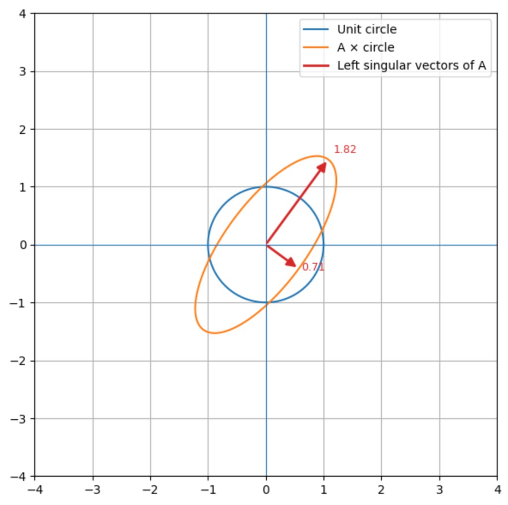
As you continue this pattern, you end up getting the $Ax_i$ vectors as the semi-axes of the ellipsoid formed by transforming the unit ball. That is, the semi-axes point in the directions of the columns of $U$ and they have magnitudes equal to the singular values of $A$. The columns of $U$ are called the left singular vectors of A. The columns of $V$ are called the right singular vectors of A.
The following shows a unit ball in $R^2$ and the ellipse created by multipling a matrix times this ball:
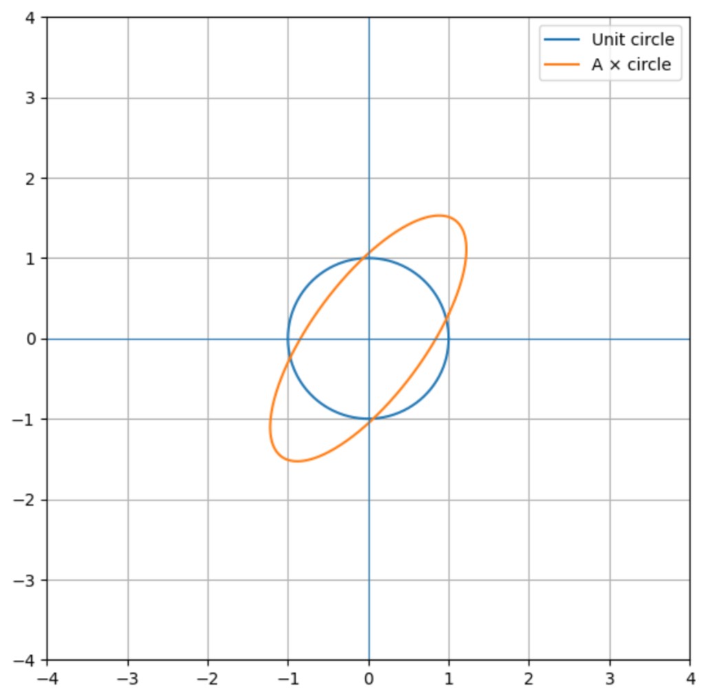
The left singular vectors of this matrix are added here, showing that they align with the semi-axes of the ellips drawn.
Now note something interesting about the volume of an ellipsoid. The volume of an ellipsoid is equal to the volume of the unit ball times the product of the lengths of the semi-axes. In $R^2$ this means that the volume is
\[\pi l_1l_2\]where $l_i$ is the length of the i’th semi axis. In $R^3$ the volume is
\[\frac{4}{3}\pi l_1l_2l_3\]In $R^n$ the volume of a unit ball is equal to:
\[\frac{\pi^\frac{n}{2}}{\Gamma(\frac{n}{2} + 1)}\]Where $\Gamma$ is the gamma function. This means the volume of an ellipsoid in $R^n$ is equal to:
\[\frac{\pi^\frac{n}{2}}{\Gamma(\frac{n}{2} + 1)} \prod_{i=1}^nl_i\]Notice what this says. This says that the ratio of the volume of the ellipsoid to the volume of the unit ball is equal to the product of lengths of the semi-axes. Since we showed using singular value decomposition that the lengths of the semi-axes are equal to the singular values of $A$, this means that this ratio is equal to the product of the singular values, which we also showed was equal to the magnitude of the determinant of $A$. So, for a unit ball $B$ and a matrix A,
\[vol(AB) = vol(B)|Det(A)|\]More surprisingly, it is actually the case that for any set $S$ of finite volume:
\[vol(AS) = vol(S) |Det(A)|\]Take a moment to think about what this means. We started off stating that the determinant was a metric for multiplicative quantity, and this makes that result crystal clear. If you take any set in $R^n$, multiply it by a matrix, and considering the volume of the resulting shape, the volume has grown by an amount equal in magnitude to the determinant of the matrix. This is a beautiful way to think about the determinant: it tells us how the matrix grows or shrinks the volume of objects.
Summary
This piece set out to provide an intuitive explanation of what the determinant is algebraically, geometrically, and philosophically. It did this by first defining the determinant. This took quite some time, as the determinant is actually a quite complicated function. We showed that it was the unique alternating m-linear function on $R^n$ which evaluates to 1 on the standard bases. We then proved several properties of the determinant. Specifically, we showed that:
\[\begin{aligned} Det(AB) &= Det(A)Det(B) \\ Det(A^T) &= Det(A) \\ Det(A) &= \prod_i \lambda_i \\ |Det(A)| &= \prod_i \sigma_i \end{aligned}\]These properties then liberated us to show how the determinant scales the volume of objects. We showed how a unit ball is transformed by a matrix, then used algebra to prove that the resulting ellipsoid has a volume equal to the ball’s volume scaled by the magnitude of the determinant. This gave us insight into what the determinant really measures: it measures a signed value of how a matrix scales the volume of a closed set.
I hope you enjoyed this. Feel free to reach out to [email protected] if you have any thoughts.