Geometric Intuition for Risk Neutral Pricing
Will Healy September 2026
Motivation
I wanted to write a piece on Stiemke’s theorem because I think it’s widely overlooked by practitioners of the fields which it touches. I’m refering particularly to the field of finance. Arbitrage pricing theory can be studied deeply without ever touching linear algebra. However, if you look at these same concepts through the lense of linear algebra, many results which originally seemed purely algebraic can be understood and visualized geometrically. I think this is quite powerful.
Prerequisites on Separability
We will rely on concepts related to separability in this piece. If you’re unfamiliar with separability, this section will give you the required prerequisites.
Separability refers to theorems and properties which make sets, points, subspaces, and objects separable, with an emphasis on linear separability. A linear separator is called a hyerplane, and is an n - 1 dimensional surface which divides an n-dimensional vector space into two halves. In $R^2$, a hyperplane is a line. In $R^3$, a hyperplane is a plane. For higher dimensions, these surfaces are hard to visualize but share the same properties. A halfspace refers to a portion of a vector space which lies on one side of a hyperplane. A hyperplane is typically defined by two values $c$ and $k$, where $c \in R^n$ and $k \in R$. It is defined as:
\[\{x | c^Tx = k\}\]The set of points whose dot product with a certain vector equals a constant draws a surface perpindicular to the vector. The value k translates that surface along the vector, with $k = 0$ having the surface pass through the origin.
A halfspace is often defined as:
\[\{x | c^Tx \leq k\}\]Replacing $\leq$ with $<$, $>$, or $\geq$ also yield valid halfspaces.
Introduction
The Gordan Stiemke theorem describes a geometrically simple yet extremely powerful result in linear algebra. It states that for any subspace whose intersection with the non-negative orthant consists of only the origin, there exists a vector $y$ strictly inside the non-negative orthant which is orthogonal to the subspace.
This piece is going to do three things. First, it’s going to make the claim this theorem is making very intuitive geometrically. Then, it is going to prove the theorem algebraically. Finally, once the theory is hopefully understood very well, it is going to use it to prove the existence of risk neutral pricing in a no-arbitrage setting. For many readers I think the geometric intuitions will be sufficient to convince them that the theorem is true. However, I encourage readers to understand of the algebraic proof. Without understanding the more rigorous proof, it will be difficult to recongize algebraic patterns where this theorem may be applicable.
Geometric Intuition on Stiemke’s Theorem
Let’s consider what this theorem is claiming in $R^2$. $R^2$ contains two classes of subspaces: lines and $R^2$ itself. Since $R^2$ obviously touches the non-negative orthant at more than just the origin, let’s consider lines.
Take any line in $R^2$ which passes through the origin. This line will either touch the non-negative orthant in infinite places, which happens in the case of a non-negative slope, or it will touch the non-negative orthant at only the origin, which happens in the case of a negative slope. Stiemke’s theorem states that in the case of a line which intersects with the non-negative orthant only at the origin, the line perpendicular to this line must go through the non-negative orthant. Equivalently, it states there is a vector strictly inside the non-negative orthant, meaning it’s values are all strictly positive, which is orthogonal to the line. That is it. The following visual shows this. The blue line is our line of choice and the red arrow is the vector in the non-negative orthant which is orthogonal to it.
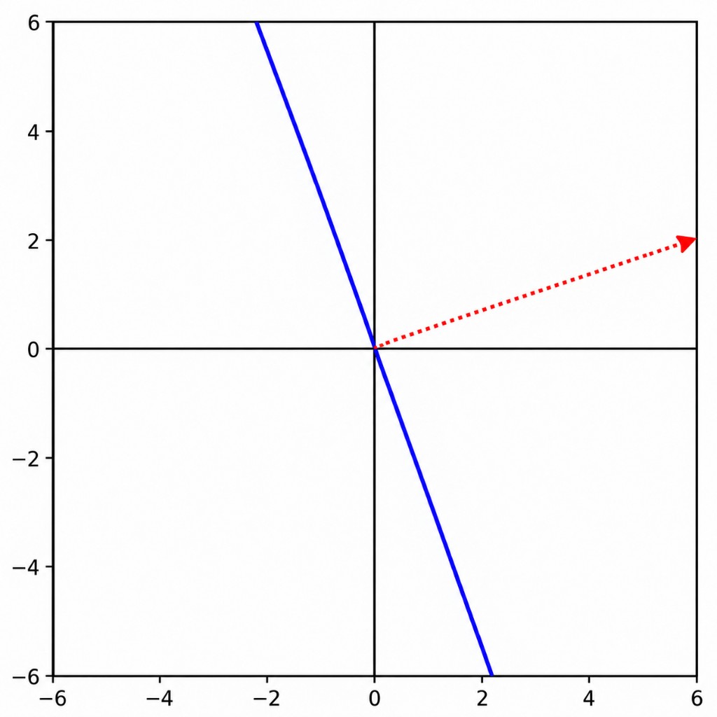
In $R^2$, Stiemke’s entire claim is that there is this red vector in the first quadrant orthogonal to the blue vector.
In $R^3$, we have a similar situation, but instead of the blue line we potentially have a plane. I say potentially because in $R^3$ a subspace can still be a line. In the case of us having a plane as our subspace, we once again have a unique line which is orthogonal to the plane. This theorem states the same thing here, that if the plane doesn’t touch the non-negative orthant other than at the origin, then the line orthogonal to it must go strictly inside the non-negative orthant.
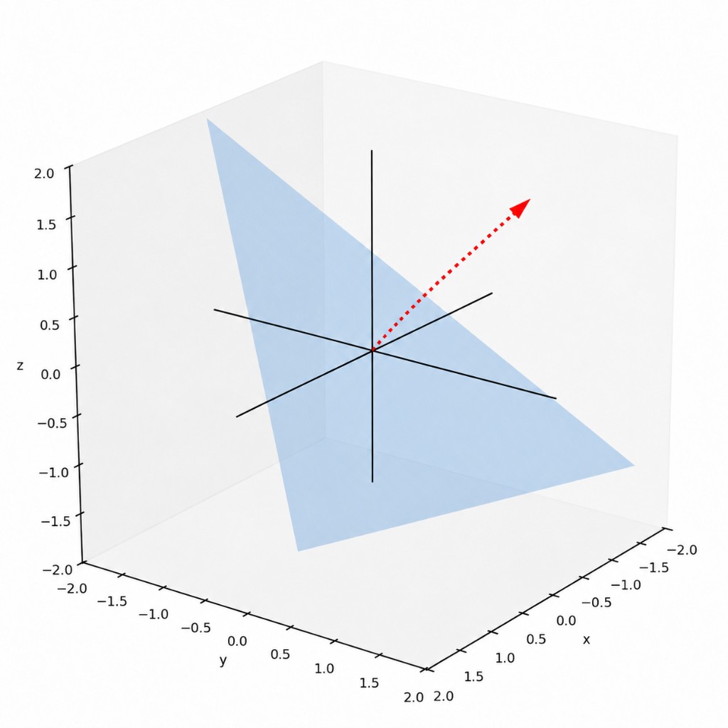
I think this result is quite intuitive when viewed geometrically in $R^3$ and in $R^2$. We will now prove this theorem algebraically for arbitrary dimensions.
Gordan Stiemke Theorem Proof
Say we have a matrix $A \in R^{m\times n}$. This matrix’s image, which defines a subspace with bases equal to the matrix’s columns, is denoted $Im(A)$. It can be defined as
\[Im(A) = \{Ax | x \in R^n\}\]Now consider the question of whether there exists a vector $y \in R^m$ such that:
\[y \neq 0\] \[y \in Im(A)\] \[y \geq 0\]Equivalently, this is asking whether the subspace defined by the image of A overlaps with the non-negative orthant anywhere but the origin. This theorem is about the implications of the case where it does not. So, let’s assume it does not.
Then, I claim there must exist $c > 0 \in R^m$ such that $A^Tc = 0$. That is, some element strictly inside the non-negative orthant must lie in the nullspace of $A^T$.
Proof of $A^Tc = 0$
First consider whether there is a separating hyperplane between the non-negative orthant and $C$. We are assuming that the only overlapping point between these two sets is at the origin. More rigourously
\[Im(A) \cap R_+^m = \{0\}\]Since $Im(A)$ and $R^m_+$ are not even disjoint, they are not strictly separable. So, rather than considering the entire non-negative orthant, let’s instead consider the separability of $Im(A)$ and the unit simplex defined as:
\[\Delta = \{x|x \geq 0, 1^Tx = 1\}\]If you’re unfamiliar with the unit simplex, it is the set of points who’s $l1$ norm is equal to 1 and whose elements are all non-negative. It is the surface of the $l1$ ball in the non-negative orthant. In \(R^2\) this is the line segment connecting $\begin{bmatrix} 1 \\ 0 \end{bmatrix}$ and $\begin{bmatrix} 0 \\ 1 \end{bmatrix}$. In \(R^3\), it looks like a triangle leaning up against a corner. It is the piece of a plane created by taking all convex combinations of $\begin{bmatrix} 1 \\ 0 \\ 0 \end{bmatrix}$, $\begin{bmatrix} 0 \\ 1 \\ 0 \end{bmatrix}$, and $\begin{bmatrix} 0 \\ 0 \\ 1 \end{bmatrix}$.
Since this simplex lies within the non-negative orthant and does not include \(\{0\}\), it must be disjoint from C. Additionally, this set is convex and compact. Two convex sets where one is closed (meaning it contains its bounds) and the other is compact (meaning it has finite bounds and contains its bounds) are strictly separable. So, since both $Im(A)$ and $\Delta$ are convex, $Im(A)$ is closed, and $\Delta$ is compact, there must exist a separating hyperplane between these two sets. That is, there must exist some $c$ and $k$ such that
\[\begin{align} \forall z \in Im(A): z^Tc - k < 0 \\ \forall \delta \in \Delta: \delta^Tc - k > 0 \end{align}\]This is equivalent to writing
\[\forall z \in Im(A): \forall \delta \in \Delta: z^Tc < \delta^Tc\]Now let’s reason about what $c$ could be. I claim $c$ must be orthogonal to every value in $Im(A)$. It’s easiest to see why using contradiction. Imagine that for some $z \in Im(A)$ it was the case that $z^Tc \neq 0$. Since $Im(A)$ is a subspace and thus closed under scalar multiplication, we could define
\[\hat{z} = z * t\]where $t$ is a huge positive scalar if $z^Tc > 0$ and a huge negative scalar if $z^Tc < 0$. By scaling $t$ we could make $\hat{z}^Tc$ arbitrarily large, at some point surpassing $\delta^Tc$. This would break our separability requirement. So, since $c$ defines our separator we’ve reached a contradiction. For this reason, any separating hyperplane must be defined by some vector $c$ such that $A^Tc = 0$. In other words, c must lie in the null space of $A^T$.
Now let’s consider the elements of $c$. I claim that they must all be strictly positive.
Proof of $c > 0$
First realize that since ${0} \in Im(A)$, the separating hyperplane must be defined by a $k > 0$. Otherwise the hyperplane would go through the origin and it would not be the case that $z^Tc - k < 0$ like is required for $z = {0}$. Additionally, since all the standard bases $e_1, e_2, … e_m$ lie inside the unit simplex, it must be the case that $e_iTc - k > 0$. Since $k > 0$, we have that:
\[\forall i: c_i = e_i^Tc > e_i^Tc - k > 0\]So $c > 0$.
Conclusion
This completes the proof of the following result:
\[Im(A) \cap R_+^m = \{0\} \rightarrow \exists c \in R^m: A^Tc = 0, c > 0\]This result, along with its converse which is also true, is called the Gordan Stiemke Theorem. We will now use this result to prove an interesting result in finance.
Risk Neutral Pricing
Imagine that we have a set of n assests and we know that in the next time step the world could be in m states. In each of these states, we know what the price of each asset would be. Now imagine that we have a payout matrix of assets:
\[A \in R^{m \times n}\]We will define $A_{ij}$ to be the price of asset j in state i one time step in the future.
One could construct a portfolio $x \in R^n$ where $x_j$ represents the quantity of asset j which we buy. $x_j$ can be positive or negative. Let’s also imagine the current price of each asset is represented by a price vector $p$, where $p_j$ represents the current price of asset j. Investing in a portfolio $x$ costs $p^Tx$ dollars. If $p^Tx$ is negative, then this means you are being paid to take on this portfolio. If $p^Tx$ is positive it means that you are paying to take on this portfolio. The value of portfolio $x$ in state i is equal to $a_i^Tx$, where $a_i$ is the i’th row of A. If for a portfolio x
\[Ax \geq 0\]Then, this portfolio is guaranteed to have a non-negative balance after one time step. If both:
\[Ax \geq 0\] \[p^Tx < 0\]are true, then this is an arbitrage opportunity, since we’re getting paid to take on a portfolio and we can’t possibly owe money at the end of the time step. Most definitions also consider
\[Ax > 0\] \[p^Tx \leq 0\]an arbitrage opportunity.
Let’s let
\[B = \begin{bmatrix} -p^T \\ A \end{bmatrix} \in R^{(m+1) \times n}\]Then, our arbitrage opportunity exists when
\[Bx = \begin{bmatrix} -p^Tx \\ Ax \end{bmatrix} \geq 0\]and
\[Bx = \begin{bmatrix} -p^Tx \\ Ax \end{bmatrix} \neq 0\]This is eqivalent to saying that there is an x such that $Bx$ is in the non-negative orthant and not at the origin. We exclude the origin since it is trivially satisfied with $x=0$ and it would not make any money. We can rewrite this condition as
\[\exists x: Bx \in R_+^{m+1} \backslash \{0\}\]Now recall our proof of the Gordan Stiemke Theorem. We proved that
\[Im(A) \cap R_+^m = \{0\} \rightarrow \exists c \in R^m: A^Tc = 0, c > 0\]Replacing A with B, we see that our arbitrage condition failing implies that there exists a $c$ such that
\[B^Tc = 0, c > 0\]Let’s let
\[c = \begin{bmatrix} a \\ \tilde{q} \end{bmatrix}\]where $a \in R_{++}$ and $\tilde{q} \in R_{++}^m$. Expanding $B^Tc$
\[B^Tc = [-p, A^T] \begin{bmatrix} a \\ \tilde{q} \end{bmatrix} = -pa + A^T\tilde{q} = 0\] \[pa = A^T\tilde{q}\]Now let us define $q = \frac{\tilde{q}}{a}$
\[p = A^Tq\]where we still know that $q > 0$.
Now imagine any reasonable asset matrix. One option you have with your money is to put it under your mattress. It will be there unchanged in the next time step. So, it is only reasonable for there to be some asset which has a payout in the next time step equal to its cost in every state. That is, some asset j such that $p_j = 1$ and the j’th column of A is a vector of 1s. Looking at the result we just derived, this would mean that for this risk free asset, we have
\[p_j = 1 = \sum_{i=1}^mq_i\]This means that the values of $q$ are all positive and sum to 1, making $q$ a probability distribution. So, these assets are all priced risk neutrally according to the probability vector $q$, where $q_j$ is the probability of ending up in state j.
This shows the following set of strong alternatives:
Either there is an arbitrage opportunity
OR
The assets are priced risk neutrally according to some probability distribution q.
Geometric Intuitions
In this setting, the column space of our matrix $A$ has one dimension for each state. A point in this space represents a specific portfolio’s value in each of these possible states. When we added $-p^T$ as a row to the matrix, one dimension then represented the negative price of the portfolio and the rest of the dimensions represented the states. Visualizing this in $R^3$ with two states we see:
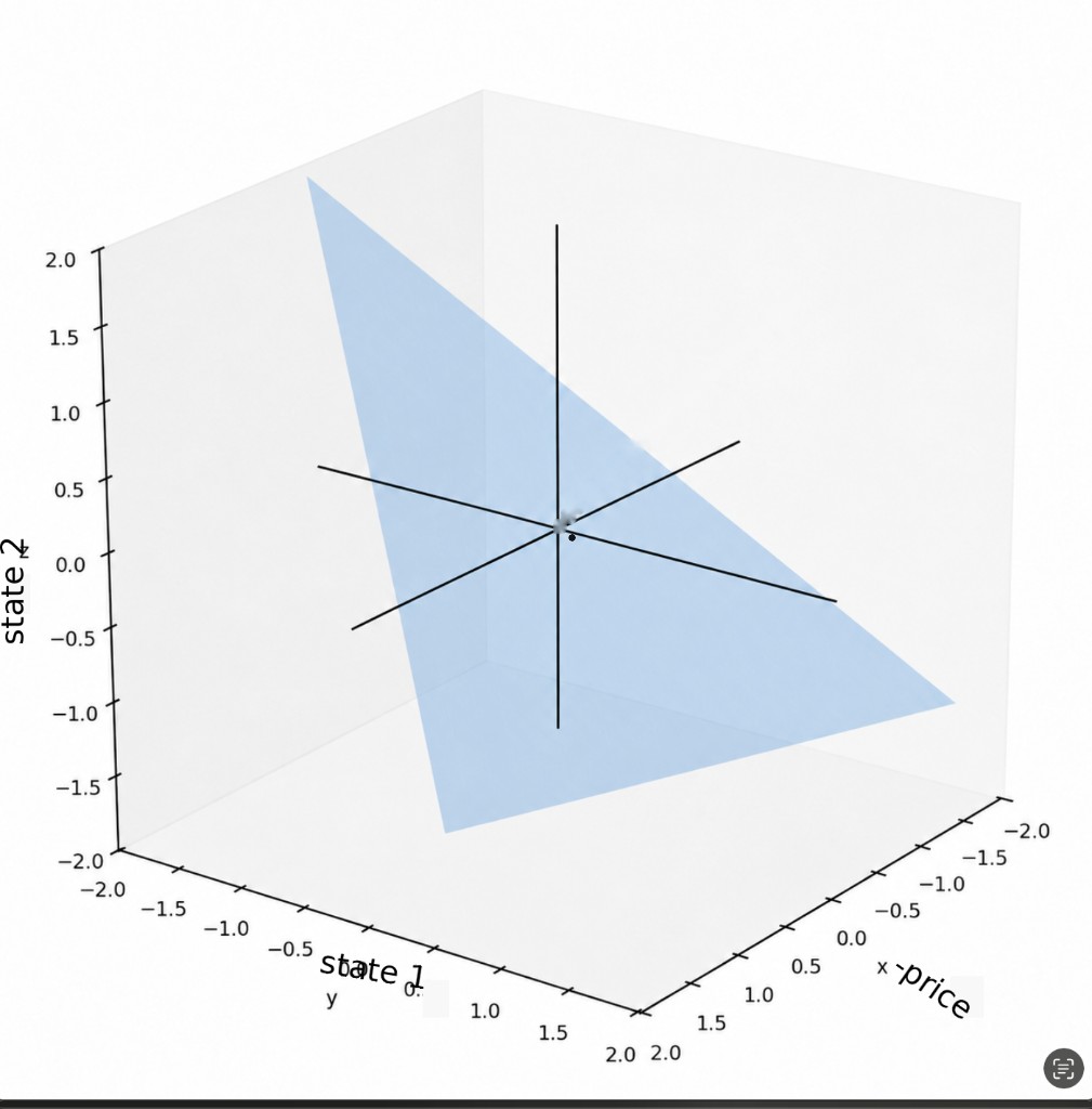
The blue plane represents the set of achievable (-price, value in state 1, value in state 2) triplets of any portfolio. Since in this example the plane doesn’t touch the non-negative orthant except for at the origin, invoking Stiemke’s theorem tells us that orthogonal to this subspace is some vector which lies strictly in the non-negative orthant. This vector contains a 1 on the dimension representing the $-p^T$ row and the risk neutral probability of landing in the state represented by each dimension for every other dimension.
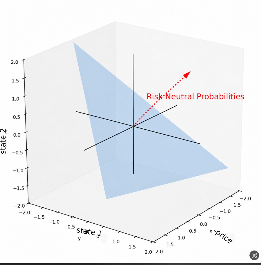
If you remember one thing from this remember the following:
For any universe of assets, if there is no arbitrage then the assets are priced risk neutrally according to a probability vector which is orthogonal to every (-price, state 1 value, state 2 value, … state m value) vector achievable by any portfolio.
I find this incredibly interesting. If anyone ever reads this I hope that they do too.